SCE-UA: Shuffle Complex Evolution Algorithm for Optimization#


![]()

![]()
SCE-UA is a lightweight Python package implementing the Shuffled Complex Evolution (SCE-UA) algorithm for global optimization. Designed primarily for hydrological model calibration, it leverages NumPy and SciPy for efficient computation and seamless integration into Python workflows.
Full documentation is available at sceua.readthedocs.io.
🌟 Features#
This implementation of the SCE-UA algorithm incorporates several major improvements from the literature over the original 1994 version. These enhancements include:
- Adaptive smoothing parameter (θ) that adjusts based on problem scale, improving numerical stability and convergence.
- Latin Hypercube Sampling (LHS) for initial population generation, ensuring better parameter space coverage compared to uniform random sampling.
- PCA-based recovery mechanism to detect and restore lost dimensions in the population.
- Best solution inclusion in every complex to accelerate convergence.
- Optimized complex evolution strategy with enhanced reflection, contraction, and mutation operations.
- Automatic parameter determination with sensible defaults based on problem dimensionality.
- Comprehensive convergence criteria, including function value tolerance, parameter tolerance, and maximum iterations.
Additionally, the package offers:
- Multithreading support for parallel objective function evaluations using threading.
- Detailed results object providing in-depth insights into the optimization process suitable for further analysis and visualization.
- Type hinting and modern Python implementation, ensuring maintainability and adherence to best coding practices.
📦 Installation#
Choose your preferred installation method:
Using pip#
Using micromamba (recommended)#
Alternatively, you can use conda or mamba.
🚀 Quick Start Guide#
The SCE-UA package has one main function called minimize, which is used to optimize a
given objective function. The API follows a similar pattern to scipy.optimize.minimize
for easy adoption.
Key Parameters#
The most important tuning parameters are n_complexes and n_points_complex
for all cases, while pca_freq and pca_tol are particularly relevant for
problems with highly correlated parameters and/or high dimensionality. Default values
are set to reasonable standards, but you can adjust them as needed for your specific
problem.
For more details, refer to the API reference.
Example Usage#
The signature for the objective function can be either:
def objective(params: FloatArray) -> float:
    """Objective function to minimize."""
    # Your implementation here
or
def objective(params: FloatArray, *args: Any) -> float:
    """Objective function to minimize."""
    # Your implementation here
where params is a NumPy array of parameters to optimize, and args is a tuple of
additional arguments to pass to the objective function. The function should return a
single floating-point value representing the objective function value.
Here's a simple example of how to use the package:
from typing import Any
import numpy as np
from numpy.typing import NDArray

import sceua

FloatArray = NDArray[np.floating[Any]]


def objective(params: FloatArray, *args: Any) -> float:
    """Objective function to minimize."""
    sim_arg1, sim_arg2, obs = args
    sim = simulation_func(params, sim_arg1, sim_arg2)
    return metric_func(sim, obs)


# Define parameter bounds as a sequence of (min, max) pairs
bounds = [(lower1, upper1), (lower2, upper2), ..., (lowerN, upperN)]

# Run optimization
result = sceua.minimize(objective, bounds, args=(sim_arg1, sim_arg2, obs), seed=42, max_workers=8)

# Access the optimization results
best_params = result.x
best_function_value = result.fun
num_iterations = result.nit
num_function_evaluations = result.nfev
Result Object#
The result object contains the following attributes:
x(numpy.ndarray): Best parameters found.fun(float): Best function value corresponding to the best parameters.nit(int): Number of iterations.nfev(int): Number of function evaluations.message(str): Message describing the termination reason.success(bool): Whether the optimization was successful.xv(numpy.ndarray): All evaluated parameter sets.funv(numpy.ndarray): Function values for all evaluated parameter sets.
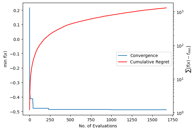
Visualization#
The result attributes can be used to create convergence plots and analyze optimization performance:
import matplotlib.pyplot as plt


_, ax1 = plt.subplots()
ax1.plot(np.minimum.accumulate(results.funv))
ax2 = ax1.twinx()
ax2.set_yscale("log")
ax2.plot(np.cumsum(results.funv - true_min), color="r")
Check the docs for more examples and API details.
📚 References#
This package is based on the following references:
- Duan, Q., Sorooshian, S., & Gupta, V. K. (1992). Effective and efficient global optimization for conceptual rainfall-runoff models. Water Resources Research, 28(4), 1015-1031. doi:10.1029/91WR02985
- Duan, Q., Gupta, V. K., & Sorooshian, S. (1994). Optimal use of the SCE-UA global optimization method for calibrating watershed models. Journal of Hydrology, 158(3-4), 265-284. doi:10.1016/0022-1694(94)90057-4
- Duan, Q., Sorooshian, S., & Gupta, V. K. (1994). A shuffled complex evolution approach for effective and efficient global minimization. Journal of optimization theory and applications, 76(3), 501-521. doi:10.1007/BF00939380
- Muttil, N., & Jayawardena, A. W. (2008). Shuffled Complex Evolution model calibrating algorithm: enhancing its robustness and efficiency. Hydrological Processes, 22(23), 4628-4638. Portico. doi:10.1002/hyp.7082
- Chu, W., Gao, X., & Sorooshian, S. (2010). Improving the shuffled complex evolution scheme for optimization of complex nonlinear hydrological systems: Application to the calibration of the Sacramento soil-moisture accounting model. Water Resources Research, 46(9). Portico. doi:10.1029/2010wr009224
Additionally, some ideas were inspired by UQPyL and SAMBO Python packages.
🤝 Contributing#
We welcome contributions! Please see the contributing section for guidelines and instructions.
📄 License#
This project is licensed under the MIT License - see the LICENSE file for details.